#COSYNE18
Tutorial
This year, we had the first tutorial session for COSYNE. From the beginning of COSYNE, there was a demand & plan for a tutorial session (according to Alex Pouget). There were 293 registered for the tutorial, and it was their first COSYNE for [155, 208] (95% CI) participants. Everybody who gave me feedback was very happy with Jonathan Pillow‘s 3.5 hour lecture (slides & code) on statistical modeling techniques for neural signals, so we are planning to run another tutorial next year at #COSYNE19 Lisbon, Portugal.
Main meeting
Basic stats: 857 registrations, 709 abstracts submitted, 396 accepted (55.8%) which was increased from 330 at Salt lake city thanks to a bigger venue at Denver (curiously, it used to be where NIPS was up till 2000).
My biased keywords of #COSYNE18: neural manifold, state space, ring attractor, recurrent neural network. Those dynamical system views are going strong.
Below are just some notes for my future self.
Tiago Branco, Computation of instinctive escape decisions (invited talk)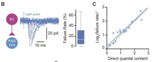
Beautiful dissecting of escape decision and response circuit in a looming dark circle task. He showed that mSC (superior colliculus) is causally involved in threat evidence representation, and the immediate downstream dPAG (periaqueductal gray) causally represents escape decision Interestingly, the synaptic connection from mSC to dPAG is weak and unreliable (fig from bioRxiv), possibly contributing to the threshold computation for escape decision.
Iain D. Couzin, Collective sensing and decision-making in animal groups: From fish schools to primate societies (Gatsby lecture)
Ian showed how he went from theoretical models of swarm behavior to virtual reality for studying interacting fish (I thought this is how you spend money in science!), how the group can solve spatial optimization problems without any individual having access to the gradient (PNAS 2009), how collective consensus can go from following strongly biased minority to a “democratized” decision making as the swarm size increased (Science 2017), and also how the collective transitions from averaging to winner take all (fig from Trends CogSci 2009).
I-80. Michael Okun, Kenneth Harris. Frequency domain structure of intrinsic infraslow dynamics of cortical microcircuits
In the time scale of tens of seconds (infraslow), they showed that inter-spike intervals alone does not, but with matching power spectral density does explain much of the slow variations. (Spikes with matching spectra and ISI were generated using a variation of amplitude adjusted Fourier transform).
I-15. Rudina Morina, Benjamin Cowley, Akash Umakantha, Adam Snyder, Matthew Smith, Byron Yu. The relationship between pairwise correlations and dimensionality reduction
From paired recordings, the spike count correlation distribution is often reported as evidence of low-dimensional activity. From population recordings, factor analysis is often used as measures of neural dimensionality. How do these two relate? Both quantities only depend on the covariance matrix, hence they investigate how the mean and standard deviation of spike count correlation (rSC) relate to dimensionality as a function of shared variance using the generative model of factor analysis. They found an interesting trend: low-dim can be either large mean rSC with small std rSC or small mean and large std (which can be shown by rotating the loadings matrix).
I-13. Lee Susman, Naama Brenner, Omri Barak. Stable memory with unstable synapses
Using anti-Hebbian learning rule  , they stored memories in limit cycles instead of stable fixed points as in traditional Hopfield networks. Also, they added a Chaotic non-stationary dynamics in the symmetric portion of the network which made the network continuously fluctuate and escape limit cycles (without losing the memory).
T-14. Emily Mackevicius, Andrew Bahle, Alex Williams, Shijie Gu, Natalia Denissenko, Mark Goldman, Michale Fee. Unsupervised discovery of neural sequences in large-scale recordings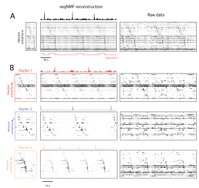
Conventional low-rank decomposition of temporal data matrix cannot find sequential structure. They have extended the convolutional non-negative matrix factorization (Non-negative Matrix Factor Deconvolution; Smaragdis 2004, 2007) for neural data, and called it SeqNMF. (MATLAB code on github; thanks for the quick bug fix @ItsNeuronal; bioRxiv 273128). It’s performance on syllable extraction and spike sequence detection was very nice.
Timothy Behrens. Building models of the world for behavioural control (invited talk)
I usually ignore fMRI talks, but the 6-fold symmetry of conceptual space was very cool. In the “canonical” bird neck & leg length space, OFC and other areas showed grid-network like signal modulations (Science 2016).
CATNIP lab had several posters on the 2nd day:
- II-2. David Hocker, Il Memming Park. Myopic control: A new control objective for neural population dynamics
- II-7. Yuan Zhao, Il Memming Park. Accessing neural states in real time: recursive variational Bayesian dual estimation
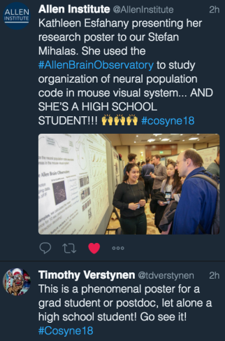
- II-62. Kathleen Esfahany, Isabel Siergiej, Yuan Zhao, Il Memming Park. Organization of neural population code in mouse visual system
Marlene Cohen. Understanding the relationship between neural variability and behavior (invited)
If correlated variability is important, it should (1) be related to performance, (2) related to individual perceptual decisions, (3) be selectively communicated between brain areas. She showed that the first principal component of noise correlation, but not the signal encoding direction, is most correlated with the choice. This was just recently published in Science 2018.
T-24. Caroline Haimerl, Eero Simoncelli. Shared stochastic modulation can facilitate biologically plausible decoding
Noise correlation tends to be in the direction of strongest decoding signal for unknown reason (Lin et al. 2015; Rabinowitz et al. 2016). They used the neural response weighted by the shared gain modulation ![]() for decoding, which was near optimal.
for decoding, which was near optimal.
Byron Yu. Brain-computer interfaces for basic science (invited)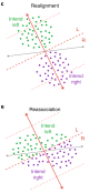
They used BCI to study how the monkey can change its output in a short time scale within the “neural manifold”. Surprisingly, the neural repertoire (distribution of possible population firing patterns) does not shift nor change in shape, but mostly reassigns meaning! (Nature Neuroscience 2018) The animal can learn out of manifold perturbation as well, but that takes days (as detailed in Emily Oby‘s talk (T-25) followed right after).
T-26. Evan Remington, Devika Narain, Eghbal Hosseini, Mehrdad Jazayeri. Control of sensorimotor dynamics through adjustment of inputs and initial condition
In a ready-set-go time interval production task with variable gain (animal has to reproduce 1.5 times the duration sometimes), the mean neural activity of the population forms a #neuralManifold. On the interval subspace, the two temporal gains produced identical mean trajectories, while on the gain subspace, they were separated. (bioRxiv 261214)
Máté Lengyel. Sampling: coding, dynamics, and computation in the cortex (invited)
If the population neural activity represents samples from the posterior, what neural dynamics would produce them (Rubin et al. 2015)? He showed that a stochastic stabilized supralinear network (SSN) with a ring architecture (not ring attractor) can sample and also reproduce neurophysiological temporal dynamics such as on/off-set response and quenching of variability (bioRxiv 2016). Also he trained an RNN to amortize inference of a simple Gaussian scale mixture model of vision, and the solution found by the RNN turns out to be non-detailed balance solution to sampling (as demonstrated by the anti-symmetric part of cross-correlation over time).
T-37. Lucas Pinto, David Tank, Carlos Brody, Stephan Thiberge. Widespread cortical involvement in evidence-based navigation
Using a transparent skull animal on Poisson towers VR decision-making task (Front. Behav. Neurosci. 2018), they found that many areas in the dorsal cortex (V1, SS, M1, RSC, mM2, aM2, etc) were correlated with accumulation of evidence. Further optogenetic inactivation of each area disrupted animal’s performance.
Vivek Jayaraman. Navigational attractor dynamics in the Drosophila brain: Going from models to mechanism (invited)
Beautiful work on the ellipsoid body–protocerebral bridge circuit and their computation involving bump attractor dynamics and path integration.
Joni Wallis. Dynamics of prefrontal computations during decision-making (invited)
Theta-oscillation phase of OFC locks to the trials when the reward criteria were linearly changing. A closed-loop microstimulation of OFC at the peak of theta disrupts learning, possibly due to disrupted theta-locked communication with hippocampus.
III-108. Rainer Engelken, Fred Wolf. A spatiotemporally-resolved view of cellular contributions to network chaos
They implemented a event-based recurrent spiking neural network that is so efficient that they can simulate a very large number (15 million) of neurons and study their dynamics. They quantified Lyapunov exponents efficiently and computed cross-correlation against the participation index.
III-75. KiJung Yoon, Xaq Pitkow. Learning nonlinearities for identifying regular structure in the brain’s inference algorithm
Loopy belief propagation often produces poor inference on non-tree graphical models. Can we do better by training a recurrent neural network to do amortized inference on graphs? The answer is yes, and it can generalize to larger networks and unseen graph structures.
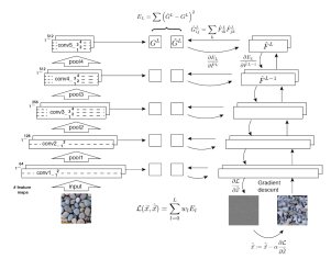
III-121. Dongsung Huh, Terrence Sejnowski. Gradient descent for spiking neural networks
They derived a differentiable synapse which gradually responses to membrane voltage near threshold. The presynaptic neuron still spikes, but the differentiable synapse allows gradient descent training of the recurrent spiking neural network. During training they can slowly make the synapse tighter and tighter to finally reach a non-differentiable synapse (arXiv 2017).
NIPS 2015 workshops
My experience during the 2 days of NIPS workshops after the main meeting (part 1,2,3).
Statistical Methods for Understanding Neural Systems workshop
 Organized by: Allie Fletcher, Jakob Macke, Ryan P. Adams, Jascha Sohl-Dickstein
Towards a theory of high dimensional, single trial neural data analysis: On the role of random projections and phase transitions
Surya Ganguli
Surya talked about conditions for recovering the embedding dimension of discrete neural responses from noisy single trial observations (very similar to his talk at NIPS 2014 workshop organized by me). He models neural response as 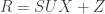


Translating between human and animal studies via Bayesian multi-task learning
Katherine Heller
Katherine talked about using a hierarchical Bayesian model and variational inference algorithms to infer linear latent dynamics. She talked about several ideas including (1) structural prior for connectivity, (2) using cross-spectral mixture kernel for LFP [Wilson & Adams ICML 2013; Ulrich et al. NISP 2015], (3) combining fMRI and LFP through shared dynamics.
Similarity matching: A new theory of neural computation
Dmitri (Mitya) Chklovskii
Principled derivation of local learning rules for PCA [Pehlevan & Chklovskii NIPS 2015] and NMF [Pehlevan & Chklovskii 2015].
Small Steps Towards Biologically Plausible Deep Learning
Yoshua Bengio
What should hidden layers do in a deep neur(on)al network? He talked about some happy coincidences: What is the objective function for STDP in this setting [Bengio et al. 2015]? Deep autoencoders and symmetric weight learning [Arora et al. 2015]. Energy based models approximates back-propagation [Bengio 2015].
The Human Visual Hierarchy is Isomorphic to the Hierarchy learned by a Deep Convolutional Neural Network Trained for Object Recognition
Pulkit Agrawal
Which layers of various CNN trained on image discrimination task explain the fMRI voxels the best? [Agrawal et al. 2014] shows hierarchy of CNN matches the visual hierarchy and it’s not because of the receptive field sizes.
Unsupervised learning with deterministic reconstruction using What-where-convnet
Yann LeCun
CNN often loses the ‘where’ information in the pooling process. What-where-convnet keeps the ‘where’ information in the pooling stage and use it to reconstruct the image [Zhao et al. 2015].
Mechanistic fallacy and modelling how we think
Neil Lawrence
He came out as a cognitive scientist. He talked about System 1 (fast subconscious data-driven inference which handles uncertainty well) and System 2 (slow conscious symbolic inference that thinks it is driving the body), and how they could talk to one another. Interesting solution to the variations of the trolly problem and how System 1 kicks in and gives the ‘irrational’ answer.
Approximation methods for inferring time-varying interactions of a large neural population (poster)
Christian Donner and Hideaki Shimazaki
Inference on an Ising model with latent diffusion dynamics on the parameters (both first and second order). Due to large number of parameters, it needs multiple trials with identical latent process to make good inference.
Panel discussion: Neil Lawrence, Yann LeCun, Yoshua Bengio, Konrad Kording, Surya Ganguli, Matthias Bethge
Discussion on the interface between neuroscience and machine learning. Are we only focusing on ‘vision’ problems too much? What problems should neuroscience focus on to help advance machine learning? How can datasets and problems change machine learning? Should we train DNN to perform more diverse tasks?
Correlations and signatures of criticality in neural population models (ML and stat physics workshop)
Jakob Macke
Jakob talked about how subsampling neural data to infer different sizes of neural dynamics could lead to misleading conclusions (esp. criticality).
Black Box Learning and Inference workshop
- Dustin Tran, Rajesh Ranganath, David M. Blei. Variational Gaussian Process. [arXiv 2015]
- Yuri Burda, Roger Grosse, Ruslan Salakhutdinov. Importance Weighted Autoencoders. [arXiv 2015]
A tighter lower-bound to the marginal likelihood! Better generative model estimation! - Alp Kucukelbir. Automatic Differentiation Variational Inference in Stan. [NIPS 2015][software]
- Jan-Willem van de Meent, David Tolpin, Brooks Paige, Frank Wood. Black-Box Policy Search with Probabilistic Programs. [arXiv 2015]
NIPS 2015 Part 3
Day 3 and 4 of NIPS main meeting (part 1, part 2). More amazing deep learning results.
Embed to control: a locally linear latent dynamics model for control from raw images
Manuel Watter, Jost Springenberg, Joschka Boedecker, Martin Riedmiller
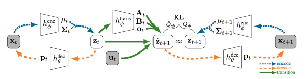 To implement optimal control in the latent state space, they used iterative Linear-Quadratic-Gaussian control applied directly to video. A gaussian latent state space was decoded from images through a deep variational latent variable model. One step prediction of latent dynamics was modeled to be locally linear where the dynamics matrices were parameterized by a neural network that depends on the current state. A variant of a variational cost that minimizes instantaneous reconstruction, and also KL divergence between predicted latent and the reconstructed latent. Deconvolution network was used, and as can be seen in the [video online], the generated images are a bit blurry, but iLQG control works well.
Deep visual analogy-making
Scott E. Reed, Yi Zhang, Yuting Zhang, Honglak Lee
 Simple vector space embedding of natural words in [Mikolov et al. NIPS 2013] showed “Madrid” – “Spain” + “France” is closest to “Paris”. Authors show that making such analogy in computer generated images is possible through a deep architecture (top figure on the right). To make an a
 nalogy of the form a : b = c : ?, first three images are encoded via f, then f(b) – f(a) + f(c), or more generally T((f(b)-f(a)), f(c)), is decoded via g to generate the output image. They trained convolutional neural network f such that T(f(b)-f(a)) is close to f(d)-f(c). Decoder with same architecture but with up-sampling instead of pooling is used for g. The performance on simple object transformation and video game character animation are quite impressive! [recorded talk]
Deep convolutional inverse graphics network
Tejas D. Kulkarni, William F. Whitney, Pushmeet Kohli, Josh Tenenbaum
 Authors propose a CNN autoencoder and training method that aims to infer ‘graphics parameters’ such as lighting and viewing angle from images. Usually the deep latent variables are hard to interpret, but here they force interpretability by training subsets of latent variables only (holding others constant) and using input with the corresponding invariance. The resulting ‘disentangled’ representation learns a meaningful approximation of a 3D graphics engine. Trained via SGVB [Kingma & Welling ICLR 2014].
Action-conditioned video prediction using deep networks in Atari games
Junhyuk Oh, Xiaoxiao Guo, Honglak Lee, Richard L. Lewis, Satinder Singh
In model based reinforcement learning, predicting the next state given the current state and action accurately is a key operation. Authors show very impressive video prediction given a couple of previous frames of Atari games and a chosen action. Hidden state is estimated using CNN, temporal correlation is learned using LSTM, and action interacts multiplicatively with the state. They used curriculum learning to make increasingly long prediction sequences with SGD + BPTT. They replaced the model-free DQN [Minh et al. NIPS 2013 workshop] with their model. See impressive results at [online videos and supplement] for yourself!
Empirical localization of homogeneous divergences on discrete sample spaces
Takashi Takenouchi, Takafumi Kanamori
![]() In many discrete probability models the (computationally intractable) normalizer for the distribution often hinders efficient estimation for high dimensional data (e.g., Ising model). Instead of using KL-divergence (equivalent to MLE) between the model and empirical distribution, if a homogeneous divergence which invariant under scaling of the underlying measure, we might be able to circumvent the difficulty. Authors use the pseudo-spherical (PS) divergence [Good, I. J. (1971)] and a trick to weight the model by the empirical distribution to make a convex optimization procedure for obtaining near MLE solution.
In many discrete probability models the (computationally intractable) normalizer for the distribution often hinders efficient estimation for high dimensional data (e.g., Ising model). Instead of using KL-divergence (equivalent to MLE) between the model and empirical distribution, if a homogeneous divergence which invariant under scaling of the underlying measure, we might be able to circumvent the difficulty. Authors use the pseudo-spherical (PS) divergence [Good, I. J. (1971)] and a trick to weight the model by the empirical distribution to make a convex optimization procedure for obtaining near MLE solution.
Equilibrated adaptive learning rates for non-convex optimization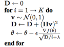
Yann Dauphin, Harm de Vries, Yoshua Bengio
Improving condition number of Hessian is important for SGD convergence speed. Authors revived equilibrated preconditioner as an adaptive learning rate for SGD.
Computational principles for deep neuronal architectures (invited talk)
Haim Sompolinsky
(1) In many early sensory systems, there’s an expansion of representation to a larger number of downstream neurons with sparser representation. This expansion ratio is around 10-100 times, and sparseness of 0.1-0.01 (fraction of neurons active). In [Babadi & Sompolinsky Neuron 2014], they derived how random connection is worse than hebbian learning for a certain scaling and sparseness constraints for representing cluster identities in the input space. (2) How about stacking such layers? Hebbian synaptic learning squashes noise as the network gets deeper. (3) Learning context-dependent influence as mixed (distributed) representation. [Mante et al. Nature 2013] is not biologically feasibly learned. Interleave sensory and context signal into deep structure with hebbian learning to solve it. (4) Extend perceptron theory for learning point clouds to manifold clouds (i.e., line segments, and L-p balls).
Efficient exact gradient update for training deep networks with very large sparse targets
Pascal Vincent, Alexandre de Brébisson, Xavier Bouthillier
If output is very high-dimensional, but sparse, as in the classification with large number of categories, the gradient computation bottleneck is the last layer. Authors propose a clever computational trick to compute gradient efficiently.
Attractor network dynamics enable preplay and rapid path planning in maze-like environments
Dane S. Corneil, Wulfram Gerstner
Hippocampal network can produce a sequence of activation (at rest) that represents goal-directed future plans. By taking the eigendecomposition of the Markov transition matrix of the maze, they obtain the ‘successor representation’ [Dayan NECO 1993] and implement it with a biologically plausible neural network.
A tractable approximation to optimal point process filtering: application to neural encoding
Yuval Harel, Ron Meir, Manfred Opper
By taking the limit of large number neurons with tuning curve centers drawn from a Gaussian, they derive a near optimal point process decoding framework. By optimizing on a grid, they derive the theoretically optimal Gaussian that minimizes MSE.
Bounding errors of expectation propagation
Guillaume P. Dehaene, Simon Barthelmé
New theory showing that EP converges faster than Laplace approximation.
Nonparametric von Mises estimators for entropies, divergences and mutual information
Kirthevasan Kandasamy, Akshay Krishnamurthy, Barnabas Poczos, Larry Wasserman, James M. Robins
Use plug-in estimator for divergences using kernel density estimator and correct for bias using von Mises expansion. It works well in low dimensions (up to 6?). [matlab code on github]
NIPS 2015 Part 2
Continuing from Part 1 (and Part 3) from Neural Information Processing Systems conference 2015 at Montreal.
Linear Response Methods for Accurate Covariance Estimates from Mean Field Variational Bayes
Ryan J. Giordano, Tamara Broderick, Michael I. Jordan
Variational inference often results in factorized forms of approximate posterior that are tighter than the exact Bayesian posterior. Authors derive a method to recover the lost covariance among parameters by perturbing the posterior. For exponential family variational distribution, a simple closed form transformation involving the Hessian of the expected log posterior. [julia code on github]
Solving Random Quadratic Systems of Equations Is Nearly as Easy as Solving Linear Systems
Yuxin Chen, Emmanuel Candes
R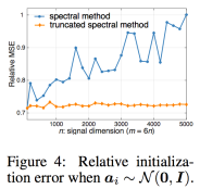 ecovering x given noisy squared measurements, e.g.,
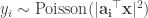

Closed-form Estimators for High-dimensional Generalized Linear Models
Eunho Yang, Aurelie C. Lozano, Pradeep K. Ravikumar
Authors derive closed-form estimators with theoretical guarantee for GLM with sparse parameter. In the high-dim regime of 


Newton-Stein Method: A Second Order Method for GLMs via Stein’s Lemma
Murat A. Erdogdu
By replacing the sum over the samples in the Hessian for GLM regression with expectation, and applying Stein’s lemma assuming Gaussian stimuli, he derived a computationally cheap 2nd order method (O(np) per iteration). This trick relies on large enough sample size 

Stochastic Expectation Propagation
Yingzhen Li, José Miguel Hernández-Lobato, Richard E. Turner
In EP, each likelihood contribution to the posterior is stored as an independent factor which is not scalable for large datasets. Authors propose to further approximate by using n copies of the same factor thus making the memory requirement of EP independent of n. This is similar to assumed density filtering (ADF) but with much better performance close to EP.
Competitive Distribution Estimation: Why is Good-Turing Good
Alon Orlitsky, Ananda Theertha Suresh
Best paper award (1 of 2). Shows theoretical near optimality of Good-Turing estimator for discrete distributions.
Learning Continuous Control Policies by Stochastic Value Gradients
Nicolas Heess, Gregory Wayne, David Silver, Tim Lillicrap, Tom Erez, Yuval Tassa
Using the reparameterization trick for continuous state space, continuous action reinforcement learning problem. [youtube video]
High-dimensional neural spike train analysis with generalized count linear dynamical systems
Yuanjun Gao, Lars Büsing, Krishna V. Shenoy, John P. Cunningham
A super flexible count distribution with neural application.
Unlocking neural population non-stationarities using hierarchical dynamics models
Mijung Park, Gergo Bohner, Jakob H. Macke
Latent processes with two time scales: one fast linear dynamics, and one slow Gaussian process.
NIPS 2015 Part 1
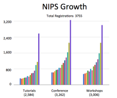 NIPS has grown to 3755 participants this year with 21.9% acceptance rate, 11% deep learning, 42 sponsors, 101 area chairs, 1524 reviewers. Here are some posters from the first night that I thought were excellent (Part 2, Part 3, workshops). They arranged the posters using KPCA axis that approximately aligned with deep-to-non-deep, so the first 40 posters or so were heavy on deep-learning. [meta blog post on other blogger’s NIPS summaries]
Deep temporal sigmoid belief networks for sequence modeling
Zhe Gan, Chunyuan Li, Ricardo Henao, David E. Carlson, Lawrence Carin
 They propose a pair of probabilistic time series models for variational inference (one generative and one recognition model) and use variance controlled log-derivative trick to do stochastic optimization. Using a binary vector, they can model an exponentially large state space, and further introduce hierarchy (deep structure) that can produce longer time scale nonlinear dependences. Each node is extremely simple: linear-logistic-Bernoulli. Zhe told he that they applied to 3-bouncing-balls video dataset represented as 900 dimensional vector, but the generated samples were not perfect and balls would often get stuck. [code on github]
Variational dropout and the local reparameterization trick [arXiv]
Diederik P. Kingma, Tim Salimans, Max Welling


They apply the SGVB reparameterization trick to parameters instead of latent variables. Most importantly, they chose a reparametrization such that the noise is independent for each observation. Upper figure (from dpkingma.com) illustrates the parameterization with slow learning due to the noise being correlated with all samples in the mini-batch, while the lower figure shows the independent form. This relates to variational interpretation of dropout, but now the dropout rate can be learned in a more principled manner.
Local expectation gradients for black box variational inference
Michalis Titsias, Miguel Lázaro-Gredilla
The two mains tricks for estimating stochastic gradient for ![E_{q(x)}[f(x)]](https://s0.wp.com/latex.php?latex=E_%7Bq%28x%29%7D%5Bf%28x%29%5D&bg=ffffff&fg=333333&s=0&c=20201002)
A recurrent latent variable model for sequential data
Junyoung Chung, Kyle Kastner, Laurent Dinh, Kratarth goel, Aaron C. Courville, Yoshua Bengio
 In conventional recurrent neural network (RNN), noise is limited to the input/output space, and the internal states are deterministic. Authors add a stochastic latent variable node to an RNN, and incorporate variational autoencoder (VAE) concepts. Latents are only time dependent through the deterministic recurrent states (with hidden LSTM units), and had a much lower dimension. They train on raw waveform of speech, and were able to generate mumbling sound that resembles the speech (I sampled their cool audio), and similarly for 2D handwriting. Their model seemed to work equally well with different complexity of observation models, unlike plain RNNs which require complex observation models to generate reasonable output. [code on github]
Texture synthesis using convolutional neural networks
Leon Gatys, Alexander S. Ecker, Matthias Bethge
 To generate texture images, they started with a deep convolutional neural network, and trained another network’s input with fixed weights until the covariance in certain layers matched. If they started with a white noise image, they could sample textures (via gradient descent optimization). [code on github]
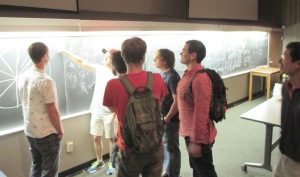
10th Black Board Day (BBD10)
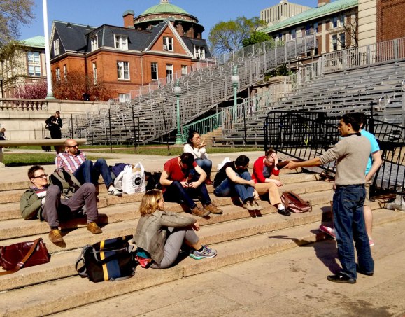
On May 2nd 2015, I organized yet another BlackBoardDay, this time in New York City (on Columbia University campus, thanks Evan!).
I started the discussion by tracing the history of modern mathematics back to Gottlob Frege (Vika pointed out the axiomatic tradition goes back to Euclid (300 BC)).
- Gottlob Frege’s Begriffsschrift, the first symbolic logic system powerful enough for mathematics (1879)
- Giuseppe Peano’s axiomatization of arithmetic (1889)
- David Hilbert’s program to build a foundation of mathematics (1900-1920s)
- Bertrand Russell’s paradox in Frege’s system (1902)
- Kurt Gödel was born! (1906)
- Russell and Whitehead’s Principia Mathematica as foundation of mathematics (1910)
- Kurt Gödel’s completeness theorem (for first-order logic) (1930)
- Kurt Gödel’s incompleteness theorem (of Principia Mathematica and related systems) (1931)
Victoria (Vika) Gitman talked about non-standard models of Peano arithmetic. She listed the first-order form of Peano axioms which is supposed to describe addition, multiplication, and ordering of natural numbers 


Ashish Myles talked about the incompleteness theorem, and other disturbing ideas. Starting from the analogy of liar’s paradox, Ashish stated that arithmetic (with multiplication) can be used to encode logical statements into natural numbers, and also write a (recursive) function that encapsulates the notion of ‘provable from axioms’. The Gödel statement G roughly says that “the natural number that encodes G is not provable”. Such statement is true (in our meta language) since if it is false, there’s a contradiction. However, either adding G or not G as an axiom to the original system is consistent. Even after including G (or “not G”) as an axiom to Peano arithmetic, there’ll be statements that are true but not provable! Vika gave an example statement that is true for natural number but is not provable from Peano axioms: all Goodstein sequence terminates at 0.
At this point, we were all feeling very cold inside, and needed some warm sunshine. So, we continued our discussion outside:
Kyle Mandli talked about Axiom of Choice (AC), which is an axiom that is somewhat counter intuitive, and independent of the Zermelo-Fraenkel (ZF) set theory: Both ZF with AC and ZF with not AC are consistent (Gödel 1964). We discussed many counter intuitive “paradoxes” as well as usefulness of AC in mathematics.
Diana Hall talked about an counter intuitive bet: suppose we have a fair coin, and we are tossing to create a sequence. Would you bet on seeing HTH first or HHT first? At first one might think they are equally likely. However, since there’s a sequence effect that makes them non-equal!
Unfortunately, due to time constraints we couldn’t talk about Uygar planed: “approximate solutions to combinatorial optimization problems implies P=NP”, hopefully we’ll hear about it on BBD11!
NIPS 2014 main meeting
NIPS is growing fast with 2400+ participants! I felt there were proportionally less “neuro” papers compared to last year, maybe because of a huge presence of deep network papers. My NIPS keywords of the year: Deep learning, Bethe approximation/partition function, variational inference, climate science, game theory, and Hamming ball. Here are my notes on the interesting papers/talks from my biased sampling by a neuroscientist as I did for the previous meetings. Other bloggers have written about the conference: Paul Mineiro, John Platt, Yisong Yue and Yun Hyokun (in Korean).
The NIPS Experiment
The program chairs, Corinna Cortes and Neil Lawrence, ran an experiment on the reviewing process and estimated the inconsistency. 10% of the papers were chosen to be reviewed independently by two pools of reviewers and area chair, hence those authors got 6-8 reviews, and had to submit 2 author responses. The disagreement was around 25%, meaning around half of the accepted papers could have been rejected (the baseline assuming independent random acceptance was around 38%). This tells you that the variability in NIPS reviewing process is, so keep that in mind whether your papers got in or not! They accepted all papers that had disagreement between the two pools, so the overall acceptance rate was a bit higher this year. For details, see Eric Price’s blog post and Bert Huang’s post.
Latent variable modeling of neural population activity
Extracting Latent Structure From Multiple Interacting Neural Populations
Joao Semedo, Amin Zandvakili, Adam Kohn, Christian K. Machens, Byron M. Yu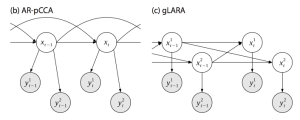
How can we quantify how two populations of neurons interact? A full interaction model would require O(N^2) which quickly makes the inference intractable. Therefore, low-dimensional interaction model could be useful, and this paper exactly does this by extending the ideas of canonical correlation analysis to vector autoregressive processes.
Clustered factor analysis of multineuronal spike data
Lars Buesing, Timothy A. Machado, John P. Cunningham, Liam Paninski
How can you put more structure to a PLDS (Poisson linear dynamical system) model? They assumed disjoint groups of neurons would have loadings from a restricted set of factors only. For application, they actually restricted the loading weights to be non-negative, in order to separate out the two underlying components of oscillation in spinal cord. They have a clever subspace clustering based initialization, and a variational inference procedure.
A Bayesian model for identifying hierarchically organised states in neural population activity
Patrick Putzky, Florian Franzen, Giacomo Bassetto, Jakob H. Macke
How do you capture discrete states in the brain, such as UP/DOWN states? They propose using a probabilistic hierarchical hidden Markov model for population of spiking neurons. The hierarchical structure reduces the effective number of parameters of the state transition matrix. The full model captures the population variability better than coupled GLMs, though the number of states and their structure is not learned. Estimation is via variational inference.
On the relations of LFPs & Neural Spike Trains
David E. Carlson, Jana Schaich Borg, Kafui Dzirasa, Lawrence Carin.
Analysis of Brain States from Multi-Region LFP Time-Series
Kyle R. Ulrich, David E. Carlson, Wenzhao Lian, Jana S. Borg, Kafui Dzirasa, Lawrence Carin
Bayesian brain, optimal brain
Fast Sampling-Based Inference in Balanced Neuronal Networks
Guillaume Hennequin, Laurence Aitchison, Mate Lengyel
Sensory Integration and Density Estimation
Joseph G. Makin, Philip N. Sabes
Optimal Neural Codes for Control and Estimation
Alex K. Susemihl, Ron Meir, Manfred Opper
Spatio-temporal Representations of Uncertainty in Spiking Neural Networks
Cristina Savin, Sophie Denève
Optimal prior-dependent neural population codes under shared input noise
Agnieszka Grabska-Barwinska, Jonathan W. Pillow
Neurons as Monte Carlo Samplers: Bayesian Inference and Learning in Spiking Networks
Yanping Huang, Rajesh P. Rao
Other Computational and/or Theoretical Neuroscience
Using the Emergent Dynamics of Attractor Networks for Computation (Posner lecture)
J. J. Hopfield
He introduced bump attractor networks via analogy of magnetic bubble (shift register) memory. He suggested that cadence and duration variations in voice can be naturally integrated with state-dependent synaptic input. Hopfield previously suggested using relative spike timings to solve a similar problem in olfaction. Note that this continuous attractor theory predicts low-dimensional neural representation. His paper is available as a preprint.
Deterministic Symmetric Positive Semidefinite Matrix Completion
William E. Bishop and Byron M. Yu
See workshop posting where Will gave a talk on this topic.
General Machine Learning
Identifying and attacking the saddle point problem in high-dimensional non-convex optimization
Yann N. Dauphin, Razvan Pascanu, Caglar Gulcehre, Kyunghyun Cho, Surya Ganguli, Yoshua Bengio
From results in statistical physics, they hypothesize that there are more saddles in high-dimension which are the main cause of slow convergence of stochastic gradient descent. In addition, exact Newton method converges to saddles, (stochastic) gradient descent is slow to get out of saddles, causing lengthy platou in training neural networks. They provide a theoretical justification for a known heuristic optimization method which is to take the absolute value of eigenvalues of the Hessian when taking the Newton step. This avoids saddles, and dramatically improves convergence speed.
A* Sampling
Chris J. Maddison, Daniel Tarlow, Tom Minka
Extends the Gumbel-Max Trick to an exact sampling algorithm for general (low-dimensional) continuous distributions with intractable normalizers. The trick involves perturbing a discrete-domain function by adding an independent samples from Gumbel distribution.They construct Gumbel process which gives bounds on the intractable log partition function, and use it to sample.
Divide-and-Conquer Learning by Anchoring a Conical Hull
Tianyi Zhou, Jeff A. Bilmes, Carlos Guestrin
Spectral Learning of Mixture of Hidden Markov Models
Cem Subakan, Johannes Traa, Paris Smaragdis
Clamping Variables and Approximate Inference
Adrian Weller, Tony Jebara
His slides are available online.
Information-based learning by agents in unbounded state spaces
Shariq A. Mobin, James A. Arnemann, Fritz Sommer
Expectation Backpropagation: Parameter-Free Training of Multilayer Neural Networks with Continuous or Discrete Weights
Daniel Soudry, Itay Hubara, Ron Meir
Self-Paced Learning with Diversity
Lu Jiang, Deyu Meng, Shoou-I Yu, Zhenzhong Lan, Shiguang Shan, Alexander Hauptmann
Last week, I co-organized the NIPS workshop titled: Large scale optical physiology: From data-acquisition to models of neural coding with Ferran Diego Andilla, Jeremy Freeman, Eftychios Pnevmatikakis and Jakob Macke. Optical neurophysiology promises larger population recordings, but we are also facing with technical challenges in hardware, software, signal processing, and statistical tools to analyze high-dimensional data. Here are highlights of some of the non-optical physiology talks:
Surya Ganguli presented exciting new results improving from his last NIPS workshop and last COSYNE workshop talks. Our experimental limitations put us to analyze severely subsampled data, and we often find correlations and low-dimensional dynamics. Surya asks “How would dynamical portraits change if we record from more neurons?” This time he had detailed results for single-trial experiments. Using matrix perturbation, random matrix, and non-commutative probability theory, they show a sharp phase transition in recoverability of the manifold. Their model was linear Gaussian, namely 
Vladimir Itskov gave a talk about inferring structural properties of the network from the estimated covariance matrix (We originally invited his collaborator Eva Pastalkova, but she couldn’t make it due to a job interview). An undirected graph which has weights that corresponds to an embedding in an Euclidean space shows a characteristic Betti curve: curve of Betti numbers as a function of threshold for the graph’s weights which is varied to construct the topological objects. For certain random graphs, the characteristics are very different, hence they used it to quantify how ‘random’ or ‘low-dimensional’ the covariances they observed were. Unfortunately, these curves are very computationally expensive so only up to 3rd Betti number can be estimated, and the Betti curves are too noisy to be used for estimating dimensionality directly. But, they found that hippocampal data were far from ‘random’. A similar talk was given at CNS 2013.
William Bishop, a 5th year graduate student working with Byron Yu and Rob Kass, talked about stitching partially overlapping covariance matrices, a problem first discussed in NIPS 2013 by Srini Turaga and coworkers: Can we estimate the full noise correlation matrix of a large population given smaller overlapping observations? He provided sufficient conditions for stitching, the most important of which is to make the covariance matrix of the overlap at least the rank of the entire covariance matrix. Furthermore, he analyzed theoretical bounds on perturbations which can be used for designing strategies for choosing the overlaps carefully. For details see the corresponding main conference paper, Deterministic Symmetric Positive Semidefinite Matrix Completion.
Unfortunately, due to weather conditions Rob Kass couldn’t make it to the workshop.
9th Black Board Day (BBD9)
![]()
Every last Sunday of April, I have been organizing a small workshop called BBD. We discuss logic, math, and science on a blackboard (this year, it was actually on a blackboard unlike the past 3 years!)
The main theme was paradox. A paradox is a puzzling contradiction; using some sort of reasoning one derives two contradicting conclusions. Consistency is an essential quality of a reasoning system, that is, it should not be able to produce contradictions by itself. Therefore, true paradoxes are hazardous to the fundamentals of being rational, but fortunately, most paradoxes are only apparent and can be resolved. Today (April 27th, 2014), we had several paradoxes presented:
Memming: I presented the Pinocchio paradox, which is a fun variant of the Liar paradox. Pinocchio’s nose grows if and only if Pinocchio tells a false statement. What happens when Pinocchio says “My nose grows now”/”My nose will grow now”? It either grows or not grows. If it grows, he is telling the truth, so it should not grow. If it is false, then it should grow, but then it is true again. Our natural language allows self-referencing, but is it really logically possible? (In the incompleteness theorem, Gödel numbering allows self-referencing using arithmetic.) There are several possible resolutions, such as, Pinocchio cannot say that statement, Pinocchio’s world is inconsistent (and hence cannot have physical reality attached to it), Pinocchio cannot know the truth value, and so on. In any case, a good logical system shouldn’t be able to produce such paradoxes.
Jonathan Pillow, continuing on the fairy tale theme, presented the sleeping beauty paradox. Toss a coin, sleeping beauty will be awakened once if it is head, twice if it is tail. Every time she is awakened, she is asked “What is your belief that the coin was heads?”, and given a drug that erases the memory of this awakening, and goes back to sleep. One argument (“halfer” position) says since a priori belief was 1/2, and each awakening does not provide more evidence, her belief does not change and would answer 1/2. The argument (“thirder” position) says that you are twice more likely to be awakened for the tail toss, hence the probability should be 1/3. If a certain reward was assigned to making a correct guess, the thirder position seems to be correct probability to use as the guess, but do we necessarily have matching belief? This paradox is still under debate, have not had a full resolution yet.
Kyle Mandi presented the classical Zeno’s paradox where your intuition on infinite sum of finite things being infinite is challenged. He also showed Gabriel’s horn where a simple (infinite) object with finite volume, but infinite surface area is given. Hence, if you were to pour in paint in this horn, you would need finite paint, but would never be able to paint the entire surface. (Hence its nickname: painter’s paradox)
Karin Knudson introduced the Banach-Tarski paradox where one solid unit sphere in 3D can be decomposed into 5 pieces, and only by translation and rotation, they are reconstructed into two solid unit spheres. In general, if two uncountable sets A, B are bounded with non-empty interior in 

 hoice (fortunately).
Harold Gutch told us about the Borel-Kolmogorov paradox. What is the conditional distribution on a great circle when points are uniformly distributed on the surface of a sphere? One argument says it should be uniform by symmetry. But, a simple sampling scheme in polar coordinate shows that it should be proportional to cosine of the angle. Basically, the lesson is, never take conditional probabilities on sets of measure zero (not to be confused with conditional densities). Furthermore, he told us about a formula to produce infinitely many paradoxes from Jaynes’ book (ch 15) based on ill-defined series convergences.
Andrew Tan presented Rosser’s extension of Gödel’s first incompleteness theorem with the statement 


I had a wonderful time, and I really appreciate my friends for joining me in this event!
Lobster olfactory scene analysis
Recently, there was a press release and a youtube video from University of Florida about one of my recent papers on neural code in the lobster olfactory system, and also by others [e.g. 1, 2, 3, 4]. I decided to write a bit about it in my own perspective. In general, I am interested in understanding how neurons process and represent information in their output through which they communicate with other neurons and collectively compute. In this paper, we show how a subset of olfactory neurons can be used like a stop watch to measure temporal patterns of smell.
Unlike vision and audition, the olfactory world is perceived through a filament of odor plume riding on top of complex and chaotic turbulence. Therefore, you are not going to be in constant contact with the odor (say the scent of freshly baked chocolate chip cookies) while you search for the source (cookies!). You might not even smell it at all for a long periods of time, even if the target is nearby depending on the air flow. Dogs are well known to be good at this task, and so are many animals. We study lobsters. Lobsters heavily rely on olfaction to track, avoid, and detect odor sources such as other lobsters, predators, and food, therefore, it is important for them to constantly analyze olfactory sensory information to put together an olfactory scene. In auditory system, the miniscule temporal differences in sound arriving to each of your ears is a critical cue for estimating the direction of the sound source. Similarly, one critical component for olfactory scene analysis is the temporal structure of the odor pattern. Therefore, we wanted to find out how neurons encode and process this information.
The neurons we study are of a subtype of olfactory sensory neurons. Sensory neurons detect signals, encode them into a temporal pattern of activity, so that it can be processed by downstream neurons. Thus, it was very surprising when we (Dr. Yuriy Bobkov) found that those neurons were spontaneously generating signals–in the form of regular bursts of action potentials–even in the absence of odor stimuli [Bobkov & Ache 2007]. We were wondering why a sensory system would generate its own signal, because the downstream neurons would not know if the signal sent by these neurons are caused by external odor stimuli (smell), or are spontaneously generated. However, we realized that they can work like little clocks. When external odor molecules stimulate the neuron, it sends a signal in a time dependent manner. Each neuron is too noisy to be a precise clock, but there is a whole population of these neurons, such that together they can measure the temporal aspects critical for the olfactory scene analysis. The temporal aspects, combined with other cues such as local flow information and navigation history, in turn can be used to track targets and estimate distances to sources. Furthermore, this temporal memory was previously believed to be formed in the brain, but our results suggest a simple yet effective mechanism in the very front end, the sensors themselves.
Applications: Currently electronic nose technology is mostly focused on discriminating ‘what’ the odor is. We bring to the table how animals might use the ‘when’ information to reconstruct the ‘where’ information, putting together an olfactory scene. Perhaps it could inspire novel search strategies for odor tracking robots. Another possibility is to build neuromorphic chips that emulate artificial neurons using the same principle to encode temporal patterns into instantaneously accessible information. This could be a part of low-power sensory processing unit in a robot. The principle we found are likely not limited to lobsters and could be shared by other animals and sensory modality.
EDIT: There’s an article on the analytical scientist about this paper.
References:
- Bobkov, Y. V. and Ache, B. W. (2007). Intrinsically bursting olfactory receptor neurons. J Neurophysiol, 97(2):1052-1057.
- Park, I. M., Bobkov, Y. V., Ache, B. W., and Príncipe, J. C. (2014). Intermittency coding in the primary olfactory system: A neural substrate for olfactory scene analysis. The Journal of Neuroscience, 34(3):941-952. [pdf]

This work by I. Memming Park is licensed under a Creative Commons Attribution 4.0 International License.
